Approximating Global Portfolio One
For all its desirable properties, GPO is quite expensive with a TER of 0.7%. This post shows how to sacrifice some convenience in order to implement a cheaper approximation. Obviously not investment advice.
Anticyclic management
Global Portfolio One (GPO) is an exchange traded equity fund that implements an interesting active strategy based on evolutionary portfolio theory, so called ultrastability in non-trivial systems. By default, companies are expected to be profitable (not even necessarily requiring unbounded growth). With a positive expectation value, we just have to make sure we can keep playing the game without getting set too far behind by unfortunate events.
In normal times GPO keeps an investment reserve of about 20%. The reserve is then invested rule based, partially in times of crisis (think MSCI World 20% below long-term high), and fully in times of escalating crisis (think MSCI World 40% below long-term high). The reserve is restored when markets recover. Note that this does not require making any predictions.
For the reserve, liquidity is paramount, even at the cost of missing out on returns or even small negative returns for this part of the portfolio. By rule of thumb, this will not underperform if it is used at least once every five years, and outperform if used more frequently. More importantly, it makes for a very safe portfolio in the long run.
For our poor man's implementation, we need some discipline to keep the reserve, and we have to rebalance when thresholds for crisis are reached. You'd have to live under a rock to miss such global events, so I don't think it is necessary to automate any particular alerts.
Diversification
Diversification is an essential part of the concept of ultrastability. In fact, ideally the portfolio should represent the entire world economy. GPO takes the closest practical approach, by investing into almost all globally investible companies (over 8000 positions). This is important to keep in mind when selecting ETFs to approximate GPO. In particular a simple MSCI World would not offer sufficient diversification.
Gleichwertprinzip
The price-earning ratio of companies depends on geography. This may be justified, but GPO simply tries to systematically collect financing costs of the world economy, so the regional allocations are adjusted. GPO ends up being a factor tilt portfolio, slightly favoring small caps and value. To implement this, GPO uses 16 ETFs, mostly in disjoint groups. That's too many to comfortably manage ourselves, so we'll go to some length to find an approximation.
The roughly 20% investment reserve is kept mostly in high quality government bonds. Unlike a large investment fund, we'll have the luxury of being able to safely use cash.
Now to approximate the the 80% in equities, something very rough like 70% MSCI All Countries World plus 10% MSCI World Small Cap would probably perform extremely similarly in most situations. But here we go ...
We will distinguish:
- North America
- 87.5% Large and mid caps
- 12.5% Small caps (based on rough approximation above)
- Japan
- Emerging Markets
- Pacific excl. Japan
- Europe and others
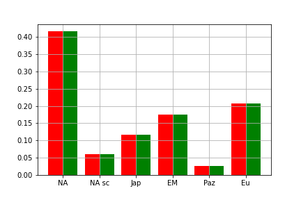
As of September 2021, aggregating all of GPOs positions, we get the following target allocation:
$$ \mathbf{g} = \begin{pmatrix} 0.416 \\ 0.059 \\ 0.117 \\ 0.175 \\ 0.026 \\ 0.206 \end{pmatrix} \begin{matrix} \textrm{North America excl. small caps} \\ \textrm{North America small caps} \\ \textrm{Japan} \\ \textrm{Emerging Markets} \\ \textrm{Pacific} \\ \textrm{Europe and others} \\ \end{matrix} $$
For Emerging Markets we'll use one of the widest possible ETFs.
- iShares Core MSCI Emerging Markets IMI UCITS ETF (Acc)
The bulk is North America, which is represented even more so in global ETFs based on market capitalization. So for now we can get away with using market cap based global ETFs, because we will have to put more (not less) weight onto other regions.
- iShares Core MSCI World UCITS ETF
- iShares MSCI World Small Cap UCITS ETF
So far there is no overlap, and we already have more than 7000 individual positions. We'll now add some overlapping regional ETFs for fine-tuning:
- Lyxor Core MSCI Japan (DR) UCITS ETF - Acc
- Xtrackers MSCI Europe Small Cap UCITS ETF 1C
Our selection can be represented as follows, ETFs in columns, regions in rows, in the order they have been introduced here.
$$ A = \begin{pmatrix} & 0.667 & & & \\ & & 0.619 & & \\ & 0.068 & 0.106 & 1 & \\ 1 & & & & \\ & 0.034 & 0.050 & & \\ & 0.191 & 0.222 & & 1 \\ \end{pmatrix} $$
Our optimization problem is now:
$$ \mathbf{x}^* = \argmin_x \| \mathbf{Ax} - \mathbf{g} \| $$
This could be solved using the ordinary least squares method. But while the constraint that the allocation vector \( \mathbf{x} \) sums to 1 may be expected to be an implicit result of the optimization, we also cannot (and do not want to) take any short positions in these ETFs:
$$ \mathbf{x} \ge 0 $$
Such a non-negative least squares problem can be converted to a quadratic program
$$ \mathbf{x}^* = \argmin_{x} \frac{1}{2} \mathbf{x}^\mathsf{T}\mathbf{Q}\mathbf{x} - \mathbf{c}^\mathsf{T}\mathbf{x} \\ \textrm{with } \mathbf{Q} = \mathbf{A}^\mathsf{T}\mathbf{A} \textrm{ and } \mathbf{c} = \mathbf{A}^\mathsf{T}\mathbf{g} \\ \textrm{such that} \begin{pmatrix} -1 & \cdots & -1 \\ 1 & \cdots & 1 \\ 1 & & \\ & \ddots & \\ & & 1 \\ \end{pmatrix} \mathbf{x} \ge \begin{pmatrix} -1 \\ 1 \\ 0 \\ \vdots \\ 0 \\ \end{pmatrix} $$
and solved, for example using quadprog.
$$ \mathbf{x}^* = \begin{pmatrix} 0.170 \\ 0.616 \\ 0.088 \\ 0.061 \\ 0.064 \\ \end{pmatrix} \begin{matrix} \textrm{MSCI EM IMI} \\ \textrm{MSCI World} \\ \textrm{MSCI World SC} \\ \textrm{Lyxor Japan} \\ \textrm{Xtrackers MSCI Europe SC} \\ \end{matrix} $$
Success. The difference between the regional allocations ( \( \mathbf{Ax}^* \) in red, \( \mathbf{g} \) in green) is barely visible.